3 R суурь ойлголтууд

Тавтай морилно уу!

Энэхүү бүлэгт бид R-ын талаарх үндсэн ойлголтуудыг авч үзнэ. Энэ нь дэлгэрэнгүй заавар болох зорилгогүй бөгөөд танд R-ын талаар анхан шатны мэдлэгийг өгч, мөн өмнө ашиглаж байсан хүмүүст ой санамжаа сэргээхэд тустай байх болно. Сургалтын материалууд хэсэгт илүү дэлгэрэнгүй сургалтын линкүүд буй.

Энэ хуудасны зарим хэсгийг R4Epis төслийн зөвшөөрлөөр бага зэрэг өөрчлөн авч ашигласан.

STATA, SAS, эсвэл Excel-ээс R руу шилжих зөвлөмжийг [R руу шилжих] хуудаснаас үзнэ үү.

3.1 Яагаад R-г ашиглана гэж?

R төслийн вэбсайтад дурдсанчлан R бол статистикийн тооцоолол, график хийхэд зориулсан програмчлалын хэл, түүний орчин юм. R нь маш уян хатан, өргөтгөх боломжтой, хөгжил нь хэрэглэгчдээрээ удирдуулдаг программ юм.

Зардал

R ашиглахад үнэгүй! Чөлөөт, нээлттэй эх сурвалжийн эргэн тойрон өндөр ёс зүйтэй байдаг.

Давтагдах чадвар

Дата менежмент, дата анализийг програмчлалын хэлээр (Excel эсвэл бусад голчлон товчлуур дээр дардаг/гараар хийдэг хэрэгслүүдтэй харьцуулахад) хийх нь давтагдах чадварыг сайжруулж, алдааг илрүүлэхэд амар болж, таны ажлын ачааллыг хөнгөвчилдөг.

Хамт олон

R хэрэглэгчдийн хамт олон маш том бөгөөд нэгэндээ үргэлж туслан хамтран ажилладаг. Амьдрал дээр тулгарч буй олон асуудлыг шийдвэрлэх шинэ багц, хэрэгслүүд өдөр бүр гарч, тэдгээрийг нь R хэрэглэгчид хэрэглэж үзэн байнга шалгаж байдаг. Үүний нэг жишээ болох R-Ladies нь дэлхий даяар салбартай, R хэрэглэгчдийн хамгийн том байгууллагуудын нэг бөгөөд гол зорилго нь R хэрэглэгчдийн дундах жендэрийн олон талт байдлыг хангах, дэмжих явдал юм. Таны ойролцоо ч салбар нь байдаг байж магадгүй!

3.2 Гол нэр томъёо

RStudio - RStudio бол R-ийг ашиглахад хялбар болгож буй хэрэглэгчийн график интерфэйс (GUI) юм. Дэлгэрэнгүйг RStudio хэсгээс уншина уу.

Объектууд - Таны R-д хадгалдаг бүх зүйл - датасетүүд, хувьсагч, тосгоны нэрсийн жагсаалт, хүн амын нийт тоо, тэр ч байтугай график гэх мэт гаралтууд - нь нэр оноогдсон объект бөгөөд тэрхүү нэрийг ашиглан дараагийн командуудад дуудаж болдог. Дэлгэрэнгүйг Объектууд хэсгээс уншина уу.

Функцууд - Функц нь оролтыг хүлээн авч, хувиргасан гаралтыг буцааж өгдөг кодын үйлдэл юм. Дэлгэрэнгүйг Функц хэсгээс уншина уу.

Багцууд - R багц гэдэг нь функцүүдийн нэгдэл юм. Дэлгэрэнгүй мэдээллийг Багц хэсгээс уншина уу.

Скриптүүд - Скрипт бол таны командуудыг агуулсан файл юм. Дэлгэрэнгүйг Скриптүүд хэсгээс уншина уу

3.3 Сургалтын материалууд

RStudio доторх материалууд

Тусламжийн баримт бичиг

R багц болон функцуудын талаархи баримт бичгийг RStudio-гийн “Help” таб дээрээс хайж болно. Энэ нь Files, Plots болон Packages бүхий хэсэгт байдаг (ихэвчлэн баруун доод хэсэгт). Хурдан хандая гэвэл та R консол дотор асуултын тэмдгийн дараа тухайн багц эсвэл функцын нэрийг бичсэнээр хамааралтай Help хуудсыг нээж болно. Ингэхдээ хаалтгүйгээр бичнэ үү.

Жишээлбэл: ?filter эсвэл ?diagrammeR.

Интерактив хичээлүүд

RStudio дотор R-ийг интерактив байдлаар сурах хэд хэдэн арга байдаг.

RStudio өөрөө learnr хэмээх R багцаар ажилладаг Tutorial хэсгийг санал болгодог. Ердөө л энэ багцыг суулгаад RStudio-ийн баруун дээд хэсэгт байрлах “Tutorial” табыг ашиглан хичээлээ нээнэ үү (Environment болон History табуудыг агуулсан хэсэг).

R багц swirlнь R консол дотор ажиллаж болох интерактив курсуудыг санал болгодог. Энэ багцыг суулгаад ачаалсны дараа R консол дээр swirl() (хоосон хаалттай) командыг ажиллуулна уу. Таны консол дээр асуулт гарч ирэх болно. Консол дээрээ бичээд хариулна уу. Ийм байдлаар таны сонгосон хичээлийг удирдан явуулах болно.

Cheatsheets

RStudio вэбсайт дээр олон PDF “cheatsheets” байдаг, жишээлбэл:

• Факторын forcats багц

• Огноо, цагийн lubridate багц

• Стрингүүдийн stringr багц

• Давтагдах үйлдлүүдэд зориулсан purrr багц

• Дата импортлох

• dplyr багцын дата хувиргах cheatsheet

• R Markdown (PDF, Word, Powerpoint гэх мэт баримт бичиг үүсгэхийн тулд)

• Shiny (интерактив вэб апп бүтээх)

• Дата зураглалын ggplot2 багц

• Картографи (GIS)

• leaflet багц (интерактив газрын зураг)

• Python-ийг R-тай хамт ашиглах (reticulate багц)

Энэ бол Excel хэрэглэгчдэд зориулагдсан онлайн материал.

Twitter

R нь маш идэвхтэй жиргээчдийн хамт олонтой бөгөөд эндээс та R-тай холбоотой төрөл бүрийн зөвлөгөө, товчлол, мэдээ авч болно. Эдгээр хаягуудыг дагана уу:

• Биднийг дагаарай! @epiRhandbook
  
• Өдөрт нэг R функц @rfuntionaday хэмээх энэ хаяг бол маш сайн мэдээлэлтэй
  
• Дата шинжлэх ухаанд R-ыг @rstats4ds
  
• RStudio @RStudio
  
• RStudio зөвлөгөөнүүд @rstudiotips
  
• R-Bloggers @Rbloggers
  
• R-ladies @RLadiesGlobal
  
• Hadley Wickham @hadleywickham

Мөн:

#epitwitter болон #rstats

Үнэгүй онлайн материалууд

Hadley Wickham, Garrett Grolemund нарын бичсэн Дата шинжлэх ухаанд R-ыг ном нь энэ чиглэлийн хамгийн гол сурах бичиг юм.

R4Epis төслийн вэбсайт нь “MSF-ийн яаралтай тусламжийн нөхцөлд тохиолддог дэгдэлтийн түгээмэл төрлүүд болон хүн амд суурилсан асуумж судалгааны дата цэвэрлэх, анализ хийх, тайлан гаргахад зориулсан стандартчилагдсан хэрэгслүүдийг боловсруулах” зорилготой юм. Та эндээс R-ын анхан шатны сургалтын материалууд, дэгдэлт, асуумж судалгааны RMarkdown тайлангийн загвар болон тэдгээрийг ашиглаж эхлэхэд туслах хичээлүүдийг олж болно.

Англи хэлээс бусад хэл

Materiales de RStudio en Español

Introduction à R et au tidyverse (Francais)

3.4 Суулгалт

R болон RStudio

R хэрхэн суулгах вэ

https://www.r-project.org/ вэбсайт руу орж өөрийн компьютерт тохирсон R-ын хамгийн сүүлийн хувилбарыг татаж авна уу.

RStudio хэрхэн суулгах вэ

https://rstudio.com/products/rstudio/download/ вэбсайт руу орж өөрийн компьютерт тохирсон RStudio-гийн хамгийн сүүлийн үеийн үнэгүй хувилбарыг татаж авна уу.

Зөвшөөрлүүд
Та R ба RStudio-г өөрийн унших (read), бичих (write) зөвшөөрөлтэй драйвт суулгах ёстойг анхаарна уу. Тэгэхгүй бол таны R багцуудыг суулгах явцад (түгээмэл тохиолддог) сөргөөр нөлөөлөх болно. Хэрэв танд асуудал тулгарвал RStudio нээх лого дээр хулганы баруун товчийг дараад “Run as administrator” сонгон нээхийг оролдоно уу. Бусад зөвлөмжийг [Сүлжээний драйв дээрх R] хуудаснаас олж болно.

R болон RStudio-г хэрхэн шинэчлэх вэ

R-ийг эхлүүлэх үед консол дээр таны R программын хувилбар харагддаг. Мөн та sessionInfo() функцийг ажиллуулан харж болно.

R-г шинэчлэхийн тулд дээр дурдсан вэбсайт руу орж R-г дахин суулгаарай. Өөрөөр installr багцын (Windows дээр) installr::updateR() функцыг ажиллуулснаар шинэчилж болно. Энэ функц нь танд хамгийн сүүлийн үеийн R хувилбарыг татаж авах, багцуудаа шинэ R хувилбар болгон шинэчлэхэд туслах харилцах цонхыг нээх болно. Дэлгэрэнгүй мэдээллийг installr баримт бичгээс олж болно.

Ингэж суулгасны дараа R-ын хуучин хувилбар таны компьютер дээр байсаар байх болно гэдгийг анхаарна уу. Та RStudio дээрх “Tools” -> “Global Options” дээр дарж R хувилбарыг сонгож R-ын хуучин хувилбарыг (хуучин “суулгац”) түр ажиллуулж болно. Энэ үйлдэл нь та R-ын хамгийн сүүлийн хувилбарт зориулан шинэчлэгдээгүй байгаа багцыг ашиглах шаардлагатай үед хэрэг болдог.

RStudio-г шинэчлэхийн тулд та дээрх вэбсайт руу орж RStudio-г дахин татаж авах боломжтой. Өөр нэг сонголт нь RStudio дотор “Help” -> “Check for Updates” дээр дарах бөгөөд гэвч энэ нь хамгийн сүүлийн үеийн шинэчлэлтийг харуулахгүй байж магадгүй.

Энэхүү гарын авлагыг бүтээхэд R, RStudio эсвэл багцуудын аль хувилбарыг ашигласан болохыг харахын тулд Редакцийн болон техникийн тэмдэглэл хуудсыг үзнэ үү.

Суулгах шаардлагатай болж магадгүй бусад програм хангамж

• TinyTeX (RMarkdown-ыг PDF болгон нэгтгэхэд зориулсан)
  
• Pandoc (RMarkdown-ыг нэгтгэхэд зориулсан)
  
• RTools (R-ын багцуудыг угсрахад зориулсан)
  
• phantomjs (халдварын гинжин хэлхээ гэх мэт хөдөлгөөнт сүлжээнүүдийн хөдөлгөөнгүй зургийг хадгалахад зориулсан)

TinyTex

TinyTex бол LaTeX-ийн custom түгээлт бөгөөд R-аас PDF үүсгэхэд хэрэгтэй байдаг. Дэлгэрэнгүй мэдээллийг https://yihui.org/tinytex/ харна уу.

R-аас TinyTex-ийг суулгахын тулд:

install.packages('tinytex')
tinytex::install_tinytex()
# TinyTeX-ийг устгахын тулд tinytex::uninstall_tinytex() ажиллуулна

Pandoc

Pandoc бол баримт бичиг хөрвүүлэгч, R-аас тусдаа програм хангамж юм. Энэ нь RStudio-той цуг ирдэг тул тусад нь татаж авах шаардлагагүй. Pandoc нь Rmarkdown-ыг .pdf гэх мэт формат руу хөрвүүлэх, комплекс үйлдлүүд хийхэд тусалдаг.

RTools

RTools бол R-д зориулсан багц үүсгэх програм хангамжийн цуглуулга юм.

Энэ вэбсайтаас суулгана: https://cran.r-project.org/bin/windows/Rtools/

phantomjs

Энэ нь ихэвчлэн вэб хуудсуудын “screenshot” авахад ашиглагддаг. Жишээлбэл, та epicontacts багц ашиглан халдварын гинжин хэлхээ хийх үед интерактив, динамик HTML файлыг гаргадаг. Хэрэв та үүнээс статик зураг авахыг хүсч байвал энэ үйл явцыг автоматжуулахын тулд webshotбагцыг ашиглаж болно. Үүний тулд “phantomjs” програм шаардлагатай. Та webshot багцаар дамжуулан webshot::install_phantomjs() командын тусламжтайгаар phantomjs-ийг суулгаж болно.

3.5 RStudio

RStudio чиг баримжаа

Эхлээд RStudio-г нээ. Тэдний лого нь хоорондоо маш төстэй харагддаг тул та R биш RStudio-г нээж байгаа эсэхээ шалгаарай.

RStudio-ийг ажиллуулахын тулд та компьютер дээрээ R суулгасан байх ёстой (суулгах зааврыг дээрээс үзнэ үү).

RStudio нь R ашиглахыг хялбарчилж буй интерфэйс юм (GUI). Та R-ыг машины хөдөлгүүр, гол ажлыг нь хийж байгаа гэж, харин RStudio-г тухайн хөдөлгүүрийг урагшлуулахад тусалдаг машины их бие (суудал, дагалдах хэрэгсэл гэх мэт) гэж ойлгож болно! Та RStudio хэрэглэгчийн интерфэйсийн бүрэн cheatsheet-ийг (PDF) эндээс үзэх боломжтой.

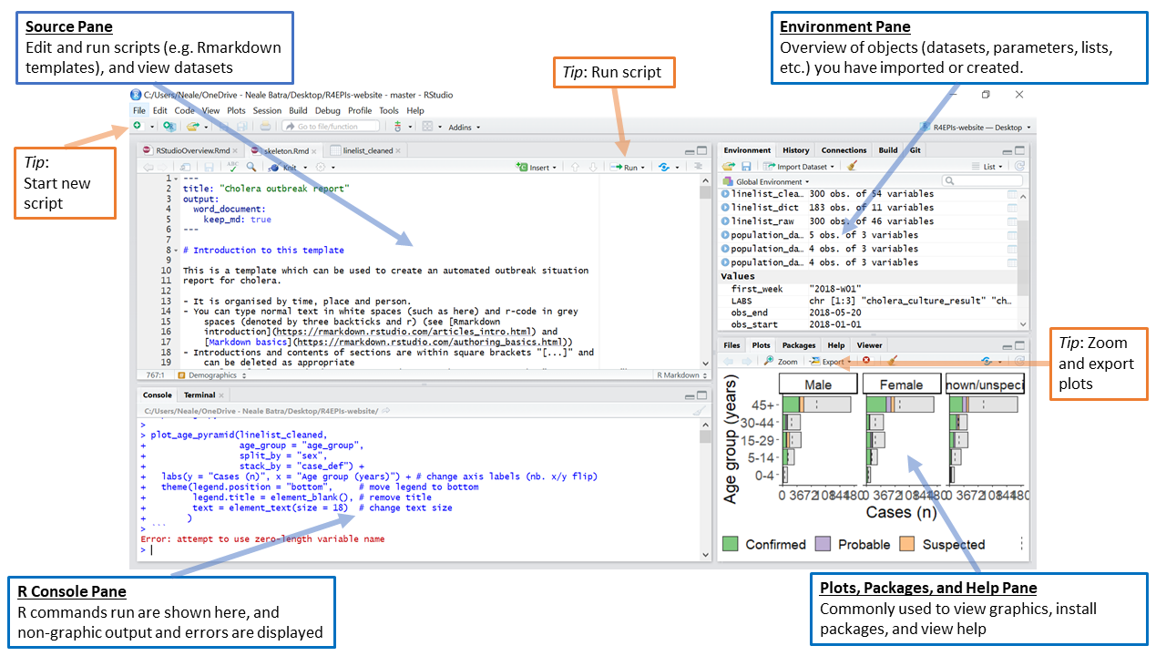
Хамгийн эхний байдлаар RStudio нь дөрвөн тэгш өнцөгт самбарыг харуулдаг.

ЗӨВЛӨГӨӨ: Хэрэв таны RStudio зүүн талдаа ганцхан дэлгэцтэй байгаа бол энэ нь та скриптүүд хараахан нээгээгүй байгаатай холбоотой юм.

Үүсвэр самбар (Source pane)
Эхний байдлаар зүүн дээд буланд байдаг энэ самбар нь скриптүүдээ засварлах, ажиллуулах, хадгалах зай юм. Скриптүүд нь таны ажиллуулахыг хүссэн командуудыг агуулдаг. Энэ самбар нь мөн датасетүүд (датафрэйм) харуулах боломжтой.

Stata хэрэглэгчдийн хувьд энэ самбар нь таны Do-file болон Data Editor цонхтой төстэй юм.

R консол самбар (Console pane)

RStudio дотор R консол нь зүүн эсвэл зүүн доод хэсэгт эхний байдлаар байрладаг бөгөөд R-ын “хөдөлгүүр”-ийн гэр юм. Энэ нь командуудын ажилладаг хэсэг бөгөөд график бус гаралт, алдаа/анхааруулах мессеж гарч ирдэг. Та R консолд командуудыг шууд оруулж ажиллуулж болох боловч скриптээс командыг ажиллуулахад хадгалагдаж үлддэг шиг эдгээр командууд хадгалагддаггүй гэдгийг ойлгоорой.

Хэрэв та Stata мэддэг бол R консол нь Command Window болон Results Window-тэй адил юм.

Орчны самбар (Environment Pane)
Програм нээгдэх үед баруун дээд буланд байдаг энэ самбарыг ихэвчлэн тухайн ажиллаж буй үеийн R-ын орчинд буй объектуудын товч мэдээллийг харахад ашигладаг. Эдгээр объектууд нь импортолсон, өөрчлөгдсөн эсвэл үүсгэсэн датасетүүд, таны тодорхойлсон параметрүүд (жишээлбэл, тухайн анализад зориулсан тодорхой эпи долоо хоног), эсвэл анализ хийх үед тодорхойлсон векторууд эсвэл листүүд (жишээлбэл, бүс нутгийн нэрс) байж болно. Та датафрэймийн нэрний хажууд байгаа сумыг дарж хувьсагчдыг нь харах боломжтой.

STATA-д энэ нь Variables Manager цонхтой хамгийн төстэй юм.

Энэ самбарт мөн өмнө нь ажиллуулсан командуудыг харах боломжтой History таб орно. Мөн та learnr багцыг суулгасан бол интерактив R хичээл хийх боломжтой “Tutorial” таб энд байдаг. Эдгээрээс гадна энэхүү самбарт гадаад холболт хийхэд зориулсан “Connections” таб, Github-тай интерфэйс хийвэл гарч ирдэг “Git” хэмээх табуудыг агуулагддаг.

Plots, Viewer, Packages, болон Help самбар

Баруун доод хэсэгт хэд хэдэн чухал табууд байдаг. Газрын зураг зэргийг багтаасан түгээмэл график дүрслэлүүдийг Plot таб дээр харуулна. Интерактив эсвэл HTML гаралтууд нь Viewer табд гарч ирнэ. Help таб нь баримт бичиг, тусламжийн файлуудыг харуулдаг. Файлын самбар нь файл нээх эсвэл устгахад зориулагдсан хөтөч юм. Packages таб нь танд R багцыг харах, суулгах, шинэчлэх, устгах, ачаалах/буулгах, танд байгаа багцын хувилбарыг харах боломжийг олгодог. Багцын талаар илүү ихийг мэдэхийг хүсвэл доорх багц хэсгээс үзнэ үү.

Энэ самбар нь Stata-гийн Plots Manager болон Project Manager цонхнуудтай төстэй мэдээлэл агуулдаг.

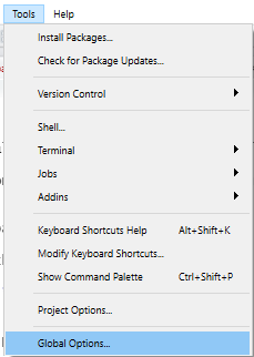
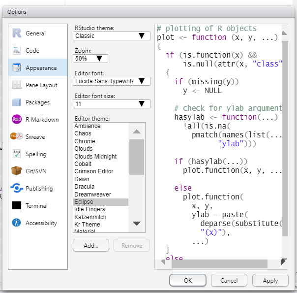
RStudio тохируулгууд

RStudio-ийн тохиргоо болон харагдах байдлыг Tools цэснээс Global Options-ийг сонгон өөрчилнө үү. Тэнд та харагдах байдал/дэвсгэр өнгө зэрэг үндсэн тохиргоонуудыг өөрчилж болно.

Дахин эхлүүлэх (Restart)

Хэрэв таны R гацвал Session цэс рүү ороод “Restart R” дээр дарж R-г дахин эхлүүлж болно. Энэ нь RStudio-г бүхэлд нь хааж, нээхээс зайлсхийдэг. Үүнийг хийснээр таны R орчинд байгаа бүх зүйл устах болно.

Гарын товчлолууд (Keyboard shortcuts)

Зарим тун хэрэгтэй гарын товчлолуудыг доор харуулав. Энэхүү RStudio хэрэглэгчийн интерфэйсийн cheatsheet-ийн хоёр дахь хуудаснаас Windows, Mac, Linux-ийн бүх гарын товчлолыг үзнэ үү.

Windows/Linux	Mac	Үйлдэл
Esc	Esc	Одоогийн командыг зогсоох (хэрэв та санамсаргүйгээр бүрэн бус командыг ажиллуулаад R консол дээр “+” тэмдэг гарчихаад байгаа үед хэрэг болдог)
Ctrl+s	Cmd+s	Хадгалах (скрипт)
Tab	Tab	Автоматаар дүүргэх
Ctrl + Enter	Cmd + Enter	Одоогийн кодын мөр(үүд)/сонголтыг ажиллуулах
Ctrl + Shift + C	Cmd + Shift + c	Тодруулсан мөрүүдэд тайлбар нэмэх/тайлбарыг арилгах
Alt + -	Option + -	<- тэмдэг оруулах
Ctrl + Shift + m	Cmd + Shift + m	%>% тэмдэг оруулах
Ctrl + l	Cmd + l	R консол цэвэрлэх
Ctrl + Alt + b	Cmd + Option + b	Эхнээс одоогийн мөр хүртэл ажиллуулах
Ctrl + Alt + t	Cmd + Option + t	Одоогийн кодын хэсгийг ажиллуулах (R Markdown)
Ctrl + Alt + i	Cmd + Shift + r	Кодын хэсэг оруулах (R Markdown руу)
Ctrl + Alt + c	Cmd + Option + c	Кодын хэсэг ажиллуулах (R Markdown)
R консолд дээшээ/доошоо сумаар	Ижил	Саяхан ажиллуулсан командуудыг сэлгэх
Скрипт дотор Shift + дээшээ/доошоо сум	Ижил	Олон кодын мөрийг сонгох
Ctrl + f	Cmd + f	Одоогийн скрипт дотор хайж олоод солих
Ctrl + Shift + f	Cmd + Shift + f	Файлуудаас хайх (олон скриптийн дунд хайх/солих)
Alt + l	Cmd + Option + l	Сонгосон кодыг хумих
Shift + Alt + l	Cmd + Shift + Option+l	Сонгосон кодыг дэлгэх

ЗӨВЛӨГӨӨ: RStudio-ийн автоматаар дүүргэх үйлдлийг ашиглахын тулд бичихдээ Tab товчлуураа ашиглана уу. Ингэснээр функцын нэрийг буруу бичихээс урьдчилан сэргийлэх боломжтой юм. Бичлэгийн дундаа Tab товчийг дарснаар одоог хүртэл бичсэн байгаа зүйл дээр үндэслэн байж болох боломжит функцууд болон объектуудын жагсаалтыг гаргана.

3.6 Функцууд

Функцууд нь R-ыг ашиглах гол цөм болдог. Функцын тусламжтайгаар та төрөл бүрийн даалгавар, үйлдлүүдийг гүйцэтгэх боломжтой болж буй юм. Нэлээд олон функцууд R-тай хамт суулгагдан ирдэг бөгөөд бусад олон функцуудыг багц хэлбэрээр татаж авах боломжтойгоос (багцууд хэсэгт тайлбарласан) гадна та өөрийн хүссэн функцээ өөрөө бичиж болно!

Энэхүү функцийн талаархи суурь ойлголтын хэсэгт дараах зүйлийг тайлбарласан болно:

• Функц гэж юу вэ, тэд хэрхэн ажилладаг талаар

• Функцын аргументууд гэж юу болох талаар

• Тодорхой функцийг ойлгоход хэрхэн тусламж авах талаар

Синтаксийн талаархи товч тэмдэглэл: Энэхүү гарын авлагад функцуудыг код-текст маягаар нээлттэй хаалт бүхий бичсэн болно, жишээ нь: filter(). Багцууд хэсэгт тайлбарласны дагуу функцуудыг багцууд дотор татаж авдаг. Энэхүү гарын авлагад багцын нэрийг dplyr гэж байгаа шиг тодоор (bold) бичсэн. Заримдаа жишээ код дээр та функцын нэрийг багцын нэртэй хоёр цэгээр (::) буюу ийм байдлаар dplyr::filter() холбон бичсэн байхыг харж болно. Энэхүү холболтын зорилгыг багцууд хэсэгт тайлбарласан.

Энгийн функцууд

Функц нь оролтыг хүлээн авч, тэдгээр оролтон дээр ямар нэгэн үйлдэл хийж, гаралт гаргадаг машинтай адил юм. Ямар гаралт байх нь тухайн функцээс хамаарна.

Функцууд нь ихэвчлэн функцын хаалтанд байрлуулсан зарим объект дээр ажилладаг. Жишээлбэл, sqrt() функц нь тооны квадрат язгуурыг тооцоолно:

sqrt(49)

## [1] 7

Мөн функцэд оруулж буй объект нь датасетийн багана байж болно (бүх төрлийн объектуудын талаар дэлгэрэнгүйг Объектууд хэсгээс үзнэ үү). R нь олон тооны датасет хадгалах боломжтой тул та датасет болон баганыг хоёуланг нь зааж өгөх хэрэгтэй. Үүнийг хийх нэг арга бол $ тэмдэглэгээг ашиглан датасетийн нэр болон баганын нэрийг (dataset$column) холбох юм. Доорх жишээн дээр linelist хэмээх датасетийн age хэмээх тоон баганыг summary() функцэд оруулснаар тухайн баганы тоон болон дутуу утгуудын хураангуй мэдээлэл гарч байна.

# 'linelist' датасетийн 'age' баганы хураангуй статистикүүдийг хэвлэх 
summary(linelist$age)

##    Min. 1st Qu.  Median    Mean 3rd Qu.    Max.    NA's 
##    0.00    6.00   13.00   16.07   23.00   84.00      86

ТЭМДЭГЛЭЛ: Хөшигний цаана функц нь хэрэглэгчдэд зориулж нэг хялбар командад багтаасан комплекс нэмэлт кодуудын бүрдэл байдаг.

Олон аргументтай функцууд

Функцууд нь ихэвчлэн таслалаар хоорондоо тусгаарлагдсан, функцын хаалтан дотор байрлах аргумент гэж нэрлэгддэг хэд хэдэн оролтыг шаарддаг.

• Зарим аргумент функцыг ажиллуулахын тулд заавал шаардлагатай байдаг бол зарим нь заавал байх шаардлагагүй

• Заавал байх шаардлагагүй аргументууд нь анхдагч утгатай байдаг

• Аргументууд нь тэмдэгт (character), тоон, логик (ҮНЭН/ХУДАЛ) болон бусад оролтыг авч болно

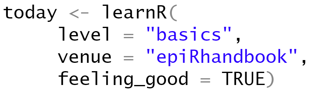
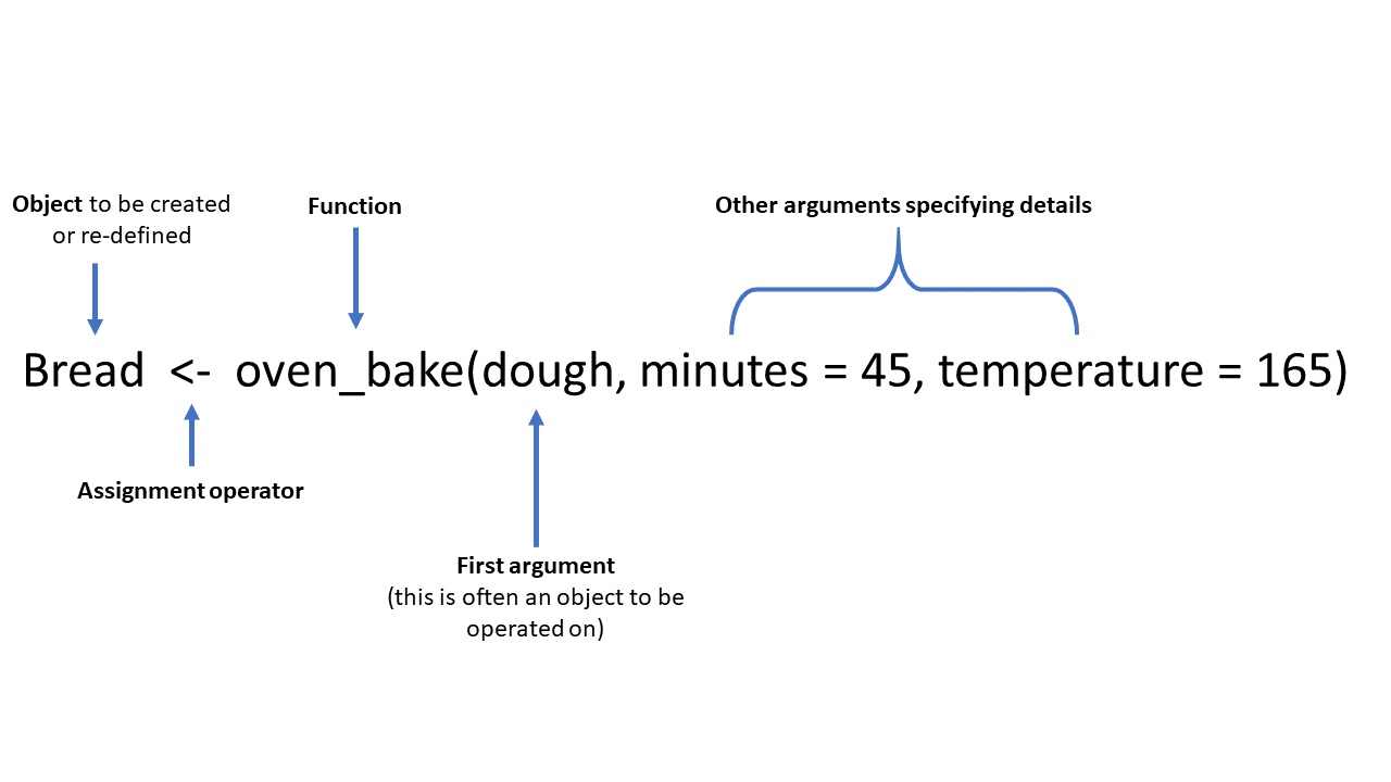
Энд ердийн функцийн жишээ болгон oven_bake() гэсэн зохиомол функц байна. Энэ функц нь оролтын объектыг (жишээлбэл, датасет эсвэл энэ жишээнд байгаа шиг “dough”) авч, нэмэлт аргументуудаар тодорхойлсон (minutes = ба temperature =) үйлдлүүдийг гүйцэтгэж байна. Гаралтыг консол дээр шууд хэвлэх эсвэл оноох операторыг (<-) ашиглан объект болгон хадгалах боломжтой .

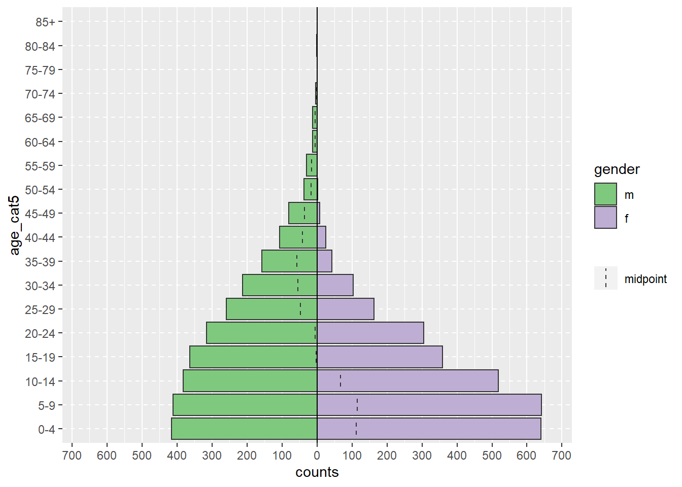
Илүү бодитой жишээ дурдвал доорхи age_pyramid() команд нь тодорхой насны бүлгүүд болон gender гэх мэт хоёртын баганууд дээр үндэслэн насны пирамидын зургийг гаргадаг. Энэхүү функцэд хаалтан дотор нь таслалаар тусгаарлагдсан гурван аргумент өгөгдсөн байна. Аргументэд өгсөн утгууд нь linelist-ийг ашиглах датафрэймээр, age_cat5-ийг тоолох баганаар, gender-ийг пирамидыг өнгөөр хуваахад ашиглах хоёртын баганаар ашиглаж байна.

# насны пирамид зурах
age_pyramid(data = linelist, age_group = "age_cat5", split_by = "gender")

Дээрх командыг аргумент бүр шинэ мөрөн дээр байх замаар урт болгон доорхтой адилаар бичиж болно. Ингэж кодоо бичих нь уншихад илүү хялбар, хэсэг тус бүрийг тайлбарлахын тулд #-тэй “тайлбар” бичихэд илүү хялбар болгодог (дэлгэрэнгүй тайлбар хийж явах нь сайн практик!). Энэхүү урт командыг ажиллуулахын тулд та тушаалыг бүхэлд нь тодруулан “Run” дээр дарах эсвэл курсороо эхний мөрөнд байрлуулаад Ctrl, Enter товчлууруудыг нэгэн зэрэг дарж болно.

# насны пирамид зурах
age_pyramid(
  data = linelist,        # тохиолдлын linelist хэрэглэх
  age_group = "age_cat5", # насны бүлгийн баганыг зааж өгөх
  split_by = "gender"     # 2 талтай пирамид зурахын тулд хүйсийн баганыг ашиглах
  )

Аргументыг тодорхой дарааллаар бичсэн тохиолдолд (функцын баримт бичигт заасны дагуу) тухайн аргументын эхний хагасыг (жишээ нь, data =) бичих шаардлагагүй. Доорх код нь дээрхтэй яг ижил пирамид үүсгэдэг, учир нь энэхүү функц нь датафрэйм, age_group хувьсагч, split_by хувьсагчийн аргументуудыг яг ийм дараалалтайгаар хүлээж байдаг.

# Энэ команд нь дээрхтэй яг ижил график үүсгэх болно
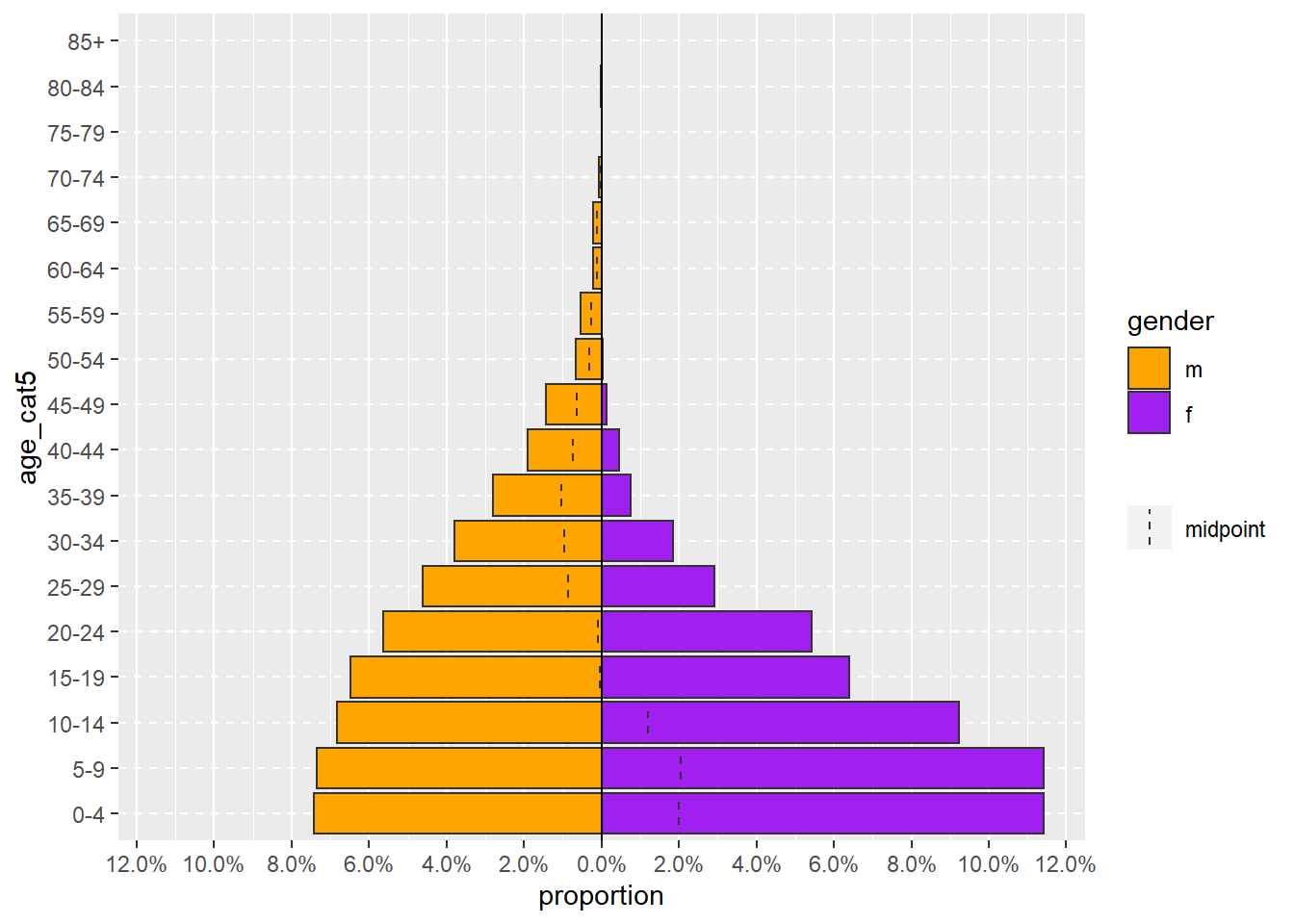
age_pyramid(linelist, "age_cat5", "gender")

Илүү комплекс age_pyramid() команд нь заавал шаардлагагүй дараахь аргументуудыг агуулж болно:

• Тооны оронд пропорцыг харуулах (анхдагч утга нь FALSE үед proportional = TRUE гэж өөрчилнө)

• Ашиглах хоёр өнгийг тодорхойлох (pal = гэдэг нь “palette” гэсэн үгийн товчлол бөгөөд хоёр өнгөний нэр бүхий вектороор хангагдсан байна. c() функц хэрхэн вектор үүсгэдэгийг объектууд хуудаснаас үзнэ үү)

ТЭМДЭГЛЭЛ: Аргументийн хоёр хэсгийг хоёуланг нь зааж өгсөн (жишээ нь proportional = TRUE) үед тухайн аргумент дарааллын хувьд хаана байрлах нь хамаагүй болно.

age_pyramid(
  linelist,                    # тохиолдлын linelist хэрэглэх
  "age_cat5",                  # насны бүлгийн багана
  "gender",                    # хүйсээр хуваах
  proportional = TRUE,         # тооны оронд хувь хэрэглэх
  pal = c("orange", "purple")  # өнгөнүүд
  )

Функц бичих

R бол функцэд чиглэсэн хэл тул та өөрийн функцийг бичих мэдлэгийг эзэмшсэн байх ёстой. Өөрөө функц бичих нь хэд хэдэн давуу талтай:

• Модульчлагдсан програмчлалыг хөнгөвчлөх - кодыг бие даасан, удирдах боломжтой хэсгүүдэд хуваадаг

• Алдаа гаргах магадлал өндөртэй байдаг давтагдсан copy, paste хийхийг орлох

• Кодын хэсгүүдэд мартагдахааргүй нэр өгөх

Функцийг хэрхэн бичих талаар Функц бичих хуудсан дээр дэлгэрэнгүй авч үзсэн болно.

3.7 Packages

Packages contain functions.

An R package is a shareable bundle of code and documentation that contains pre-defined functions. Users in the R community develop packages all the time catered to specific problems, it is likely that one can help with your work! You will install and use hundreds of packages in your use of R.

On installation, R contains “base” packages and functions that perform common elementary tasks. But many R users create specialized functions, which are verified by the R community and which you can download as a package for your own use. In this handbook, package names are written in bold. One of the more challenging aspects of R is that there are often many functions or packages to choose from to complete a given task.

Install and load

Functions are contained within packages which can be downloaded (“installed”) to your computer from the internet. Once a package is downloaded, it is stored in your “library”. You can then access the functions it contains during your current R session by “loading” the package.

Think of R as your personal library: When you download a package, your library gains a new book of functions, but each time you want to use a function in that book, you must borrow (“load”) that book from your library.

In summary: to use the functions available in an R package, 2 steps must be implemented:

1. The package must be installed (once), and
   
2. The package must be loaded (each R session)

Your library

Your “library” is actually a folder on your computer, containing a folder for each package that has been installed. Find out where R is installed in your computer, and look for a folder called “win-library”. For example: R\win-library\4.0 (the 4.0 is the R version - you’ll have a different library for each R version you’ve downloaded).

You can print the file path to your library by entering .libPaths() (empty parentheses). This becomes especially important if working with R on network drives.

Install from CRAN

Most often, R users download packages from CRAN. CRAN (Comprehensive R Archive Network) is an online public warehouse of R packages that have been published by R community members.

Are you worried about viruses and security when downloading a package from CRAN? Read this article on the topic.

How to install and load

In this handbook, we suggest using the pacman package (short for “package manager”). It offers a convenient function p_load() which will install a package if necessary and load it for use in the current R session.

The syntax quite simple. Just list the names of the packages within the p_load() parentheses, separated by commas. This command will install the rio, tidyverse, and here packages if they are not yet installed, and will load them for use. This makes the p_load() approach convenient and concise if sharing scripts with others. Note that package names are case-sensitive.

# Install (if necessary) and load packages for use
pacman::p_load(rio, tidyverse, here)

Note that we have used the syntax pacman::p_load() which explicitly writes the package name (pacman) prior to the function name (p_load()), connected by two colons ::. This syntax is useful because it also loads the pacman package (assuming it is already installed).

There are alternative base R functions that you will see often. The base R function for installing a package is install.packages(). The name of the package to install must be provided in the parentheses in quotes. If you want to install multiple packages in one command, they must be listed within a character vector c().

Note: this command installs a package, but does not load it for use in the current session.

# install a single package with base R
install.packages("tidyverse")

# install multiple packages with base R
install.packages(c("tidyverse", "rio", "here"))

Installation can also be accomplished point-and-click by going to the RStudio “Packages” pane and clicking “Install” and searching for the desired package name.

The base R function to load a package for use (after it has been installed) is library(). It can load only one package at a time (another reason to use p_load()). You can provide the package name with or without quotes.

# load packages for use, with base R
library(tidyverse)
library(rio)
library(here)

To check whether a package in installed and/or loaded, you can view the Packages pane in RStudio. If the package is installed, it is shown there with version number. If its box is checked, it is loaded for the current session.

Install from Github

Sometimes, you need to install a package that is not yet available from CRAN. Or perhaps the package is available on CRAN but you want the development version with new features not yet offered in the more stable published CRAN version. These are often hosted on the website github.com in a free, public-facing code “repository”. Read more about Github in the handbook page on Version control and collaboration with Git and Github.

To download R packages from Github, you can use the function p_load_gh() from pacman, which will install the package if necessary, and load it for use in your current R session. Alternatives to install include using the remotes or devtools packages. Read more about all the pacman functions in the package documentation.

To install from Github, you have to provide more information. You must provide:

1. The Github ID of the repository owner
2. The name of the repository that contains the package
   
3. (optional) The name of the “branch” (specific development version) you want to download

In the examples below, the first word in the quotation marks is the Github ID of the repository owner, after the slash is the name of the repository (the name of the package).

# install/load the epicontacts package from its Github repository
p_load_gh("reconhub/epicontacts")

If you want to install from a “branch” (version) other than the main branch, add the branch name after an “@”, after the repository name.

# install the "timeline" branch of the epicontacts package from Github
p_load_gh("reconhub/epicontacts@timeline")

If there is no difference between the Github version and the version on your computer, no action will be taken. You can “force” a re-install by instead using p_load_current_gh() with the argument update = TRUE. Read more about pacman in this online vignette

Install from ZIP or TAR

You could install the package from a URL:

packageurl <- "https://cran.r-project.org/src/contrib/Archive/dsr/dsr_0.2.2.tar.gz"
install.packages(packageurl, repos=NULL, type="source")

Or, download it to your computer in a zipped file:

Option 1: using install_local() from the remotes package

remotes::install_local("~/Downloads/dplyr-master.zip")

Option 2: using install.packages() from base R, providing the file path to the ZIP file and setting type = "source and repos = NULL.

install.packages("~/Downloads/dplyr-master.zip", repos=NULL, type="source")

Code syntax

For clarity in this handbook, functions are sometimes preceded by the name of their package using the :: symbol in the following way: package_name::function_name()

Once a package is loaded for a session, this explicit style is not necessary. One can just use function_name(). However writing the package name is useful when a function name is common and may exist in multiple packages (e.g. plot()). Writing the package name will also load the package if it is not already loaded.

# This command uses the package "rio" and its function "import()" to import a dataset
linelist <- rio::import("linelist.xlsx", which = "Sheet1")

Function help

To read more about a function, you can search for it in the Help tab of the lower-right RStudio. You can also run a command like ?thefunctionname (put the name of the function after a question mark) and the Help page will appear in the Help pane. Finally, try searching online for resources.

Update packages

You can update packages by re-installing them. You can also click the green “Update” button in your RStudio Packages pane to see which packages have new versions to install. Be aware that your old code may need to be updated if there is a major revision to how a function works!

Delete packages

Use p_delete() from pacman, or remove.packages() from base R. Alternatively, go find the folder which contains your library and manually delete the folder.

Dependencies

Packages often depend on other packages to work. These are called dependencies. If a dependency fails to install, then the package depending on it may also fail to install.

See the dependencies of a package with p_depends(), and see which packages depend on it with p_depends_reverse()

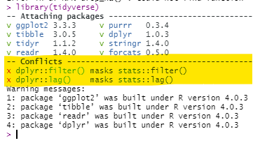
Masked functions

It is not uncommon that two or more packages contain the same function name. For example, the package dplyr has a filter() function, but so does the package stats. The default filter() function depends on the order these packages are first loaded in the R session - the later one will be the default for the command filter().

You can check the order in your Environment pane of R Studio - click the drop-down for “Global Environment” and see the order of the packages. Functions from packages lower on that drop-down list will mask functions of the same name in packages that appear higher in the drop-down list. When first loading a package, R will warn you in the console if masking is occurring, but this can be easy to miss.

Here are ways you can fix masking:

1. Specify the package name in the command. For example, use dplyr::filter()
   
2. Re-arrange the order in which the packages are loaded (e.g. within p_load()), and start a new R session

Detach / unload

To detach (unload) a package, use this command, with the correct package name and only one colon. Note that this may not resolve masking.

detach(package:PACKAGE_NAME_HERE, unload=TRUE)

Install older version

See this guide to install an older version of a particular package.

Suggested packages

See the page on Suggested packages for a listing of packages we recommend for everyday epidemiology.

3.8 Scripts

Scripts are a fundamental part of programming. They are documents that hold your commands (e.g. functions to create and modify datasets, print visualizations, etc). You can save a script and run it again later. There are many advantages to storing and running your commands from a script (vs. typing commands one-by-one into the R console “command line”):

• Portability - you can share your work with others by sending them your scripts
  
• Reproducibility - so that you and others know exactly what you did
  
• Version control - so you can track changes made by yourself or colleagues
  
• Commenting/annotation - to explain to your colleagues what you have done

Commenting

In a script you can also annotate (“comment”) around your R code. Commenting is helpful to explain to yourself and other readers what you are doing. You can add a comment by typing the hash symbol (#) and writing your comment after it. The commented text will appear in a different color than the R code.

Any code written after the # will not be run. Therefore, placing a # before code is also a useful way to temporarily block a line of code (“comment out”) if you do not want to delete it). You can comment out/in multiple lines at once by highlighting them and pressing Ctrl+Shift+c (Cmd+Shift+c in Mac).

# A comment can be on a line by itself
# import data
linelist <- import("linelist_raw.xlsx") %>%   # a comment can also come after code
# filter(age > 50)                          # It can also be used to deactivate / remove a line of code
  count()

• Comment on what you are doing and on why you are doing it.
  
• Break your code into logical sections
  
• Accompany your code with a text step-by-step description of what you are doing (e.g. numbered steps)

Style

It is important to be conscious of your coding style - especially if working on a team. We advocate for the tidyverse style guide. There are also packages such as styler and lintr which help you conform to this style.

A few very basic points to make your code readable to others:
* When naming objects, use only lowercase letters, numbers, and underscores _, e.g. my_data
* Use frequent spaces, including around operators, e.g. n = 1 and age_new <- age_old + 3

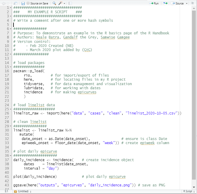
Example Script

Below is an example of a short R script. Remember, the better you succinctly explain your code in comments, the more your colleagues will like you!

R markdown

An R markdown script is a type of R script in which the script itself becomes an output document (PDF, Word, HTML, Powerpoint, etc.). These are incredibly useful and versatile tools often used to create dynamic and automated reports. Even this website and handbook is produced with R markdown scripts!

It is worth noting that beginner R users can also use R Markdown - do not be intimidated! To learn more, see the handbook page on Reports with R Markdown documents.

R notebooks

There is no difference between writing in a Rmarkdown vs an R notebook. However the execution of the document differs slightly. See this site for more details.

Shiny

Shiny apps/websites are contained within one script, which must be named app.R. This file has three components:

1. A user interface (ui)
   
2. A server function
   
3. A call to the shinyApp function

See the handbook page on Dashboards with Shiny, or this online tutorial: Shiny tutorial

In older times, the above file was split into two files (ui.R and server.R)

Code folding

You can collapse portions of code to make your script easier to read.

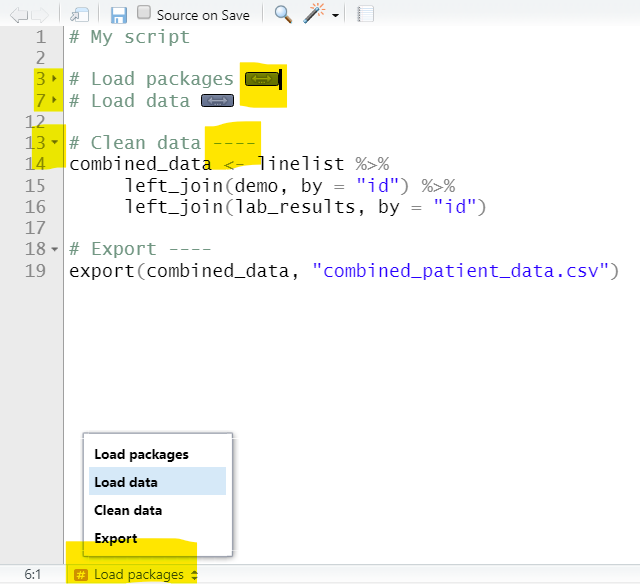
To do this, create a text header with #, write your header, and follow it with at least 4 of either dashes (-), hashes (#) or equals (=). When you have done this, a small arrow will appear in the “gutter” to the left (by the row number). You can click this arrow and the code below until the next header will collapse and a dual-arrow icon will appear in its place.

To expand the code, either click the arrow in the gutter again, or the dual-arrow icon. There are also keyboard shortcuts as explained in the RStudio section of this page.

By creating headers with #, you will also activate the Table of Contents at the bottom of your script (see below) that you can use to navigate your script. You can create sub-headers by adding more # symbols, for example # for primary, ## for seconary, and ### for tertiary headers.

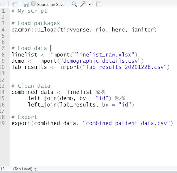
Below are two versions of an example script. On the left is the original with commented headers. On the right, four dashes have been written after each header, making them collapsible. Two of them have been collapsed, and you can see that the Table of Contents at the bottom now shows each section.

Other areas of code that are automatically eligible for folding include “braced” regions with brackets { } such as function definitions or conditional blocks (if else statements). You can read more about code folding at the RStudio site.

3.9 Working directory

The working directory is the root folder location used by R for your work - where R looks for and saves files by default. By default, it will save new files and outputs to this location, and will look for files to import (e.g. datasets) here as well.

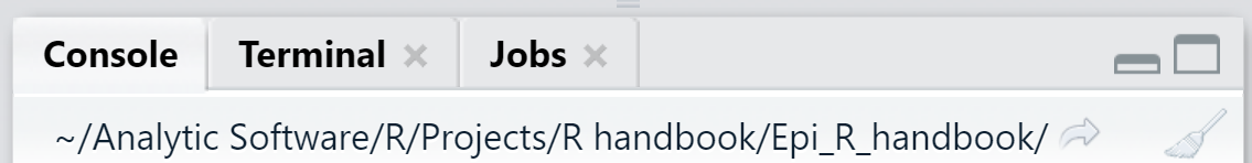
The working directory appears in grey text at the top of the RStudio Console pane. You can also print the current working directory by running getwd() (leave the parentheses empty).

Recommended approach

See the page on [R projects] for details on our recommended approach to managing your working directory.
A common, efficient, and trouble-free way to manage your working directory and file paths is to combine these 3 elements in an [R project][R projects]-oriented workflow:

1. An R Project to store all your files (see page on [R projects])
   
2. The here package to locate files (see page on [Import and export])
   
3. The rio package to import/export files (see page on [Import and export])

Set by command

Until recently, many people learning R were taught to begin their scripts with a setwd() command. Please instead consider using an [R project][R projects]-oriented workflow and read the reasons for not using setwd(). In brief, your work becomes specific to your computer, file paths used to import and export files become “brittle”, and this severely hinders collaboration and use of your code on any other computer. There are easy alternatives!

As noted above, although we do not recommend this approach in most circumstances, you can use the command setwd() with the desired folder file path in quotations, for example:

setwd("C:/Documents/R Files/My analysis")

DANGER: Setting a working directory with setwd() can be “brittle” if the file path is specific to one computer. Instead, use file paths relative to an R Project root directory (with the here package).

Set manually

To set the working directory manually (the point-and-click equivalent of setwd()), click the Session drop-down menu and go to “Set Working Directory” and then “Choose Directory”. This will set the working directory for that specific R session. Note: if using this approach, you will have to do this manually each time you open RStudio.

Within an R project

If using an R project, the working directory will default to the R project root folder that contains the “.rproj” file. This will apply if you open RStudio by clicking open the R Project (the file with “.rproj” extension).

Working directory in an R markdown

In an R markdown script, the default working directory is the folder the Rmarkdown file (.Rmd) is saved within. If using an R project and here package, this does not apply and the working directory will be here() as explained in the [R projects] page.

If you want to change the working directory of a stand-alone R markdown (not in an R project), if you use setwd() this will only apply to that specific code chunk. To make the change for all code chunks in an R markdown, edit the setup chunk to add the root.dir = parameter, such as below:

knitr::opts_knit$set(root.dir = 'desired/directorypath')

It is much easier to just use the R markdown within an R project and use the here package.

Providing file paths

Perhaps the most common source of frustration for an R beginner (at least on a Windows machine) is typing in a file path to import or export data. There is a thorough explanation of how to best input file paths in the [Import and export] page, but here are a few key points:

Broken paths

Below is an example of an “absolute” or “full address” file path. These will likely break if used by another computer. One exception is if you are using a shared/network drive.

C:/Users/Name/Document/Analytic Software/R/Projects/Analysis2019/data/March2019.csv  

Slash direction

If typing in a file path, be aware the direction of the slashes. Use forward slashes (/) to separate the components (“data/provincial.csv”). For Windows users, the default way that file paths are displayed is with back slashes (\) - so you will need to change the direction of each slash. If you use the here package as described in the [R projects] page the slash direction is not an issue.

Relative file paths

We generally recommend providing “relative” filepaths instead - that is, the path relative to the root of your R Project. You can do this using the here package as explained in the [R projects] page. A relativel filepath might look like this:

# Import csv linelist from the data/linelist/clean/ sub-folders of an R project
linelist <- import(here("data", "clean", "linelists", "marin_country.csv"))

Even if using relative file paths within an R project, you can still use absolute paths to import/export data outside your R project.

3.10 Objects

Everything in R is an object, and R is an “object-oriented” language. These sections will explain:

• How to create objects (<-)
• Types of objects (e.g. data frames, vectors..)
  
• How to access subparts of objects (e.g. variables in a dataset)
  
• Classes of objects (e.g. numeric, logical, integer, double, character, factor)

Everything is an object

This section is adapted from the R4Epis project.
Everything you store in R - datasets, variables, a list of village names, a total population number, even outputs such as graphs - are objects which are assigned a name and can be referenced in later commands.

An object exists when you have assigned it a value (see the assignment section below). When it is assigned a value, the object appears in the Environment (see the upper right pane of RStudio). It can then be operated upon, manipulated, changed, and re-defined.

Defining objects (<-)

Create objects by assigning them a value with the <- operator.
You can think of the assignment operator <- as the words “is defined as”. Assignment commands generally follow a standard order:

object_name <- value (or process/calculation that produce a value)

For example, you may want to record the current epidemiological reporting week as an object for reference in later code. In this example, the object current_week is created when it is assigned the value "2018-W10" (the quote marks make this a character value). The object current_week will then appear in the RStudio Environment pane (upper-right) and can be referenced in later commands.

See the R commands and their output in the boxes below.

current_week <- "2018-W10"   # this command creates the object current_week by assigning it a value
current_week                 # this command prints the current value of current_week object in the console

## [1] "2018-W10"

NOTE: Note the [1] in the R console output is simply indicating that you are viewing the first item of the output

CAUTION: An object’s value can be over-written at any time by running an assignment command to re-define its value. Thus, the order of the commands run is very important.

The following command will re-define the value of current_week:

current_week <- "2018-W51"   # assigns a NEW value to the object current_week
current_week                 # prints the current value of current_week in the console

## [1] "2018-W51"

Equals signs =

You will also see equals signs in R code:

• A double equals sign == between two objects or values asks a logical question: “is this equal to that?”.
  
• You will also see equals signs within functions used to specify values of function arguments (read about these in sections below), for example max(age, na.rm = TRUE).
  
• You can use a single equals sign = in place of <- to create and define objects, but this is discouraged. You can read about why this is discouraged here.

Datasets

Datasets are also objects (typically “dataframes”) and must be assigned names when they are imported. In the code below, the object linelist is created and assigned the value of a CSV file imported with the rio package and its import() function.

# linelist is created and assigned the value of the imported CSV file
linelist <- import("my_linelist.csv")

You can read more about importing and exporting datasets with the section on [Import and export].

CAUTION: A quick note on naming of objects:

• Object names must not contain spaces, but you should use underscore (_) or a period (.) instead of a space.
  
• Object names are case-sensitive (meaning that Dataset_A is different from dataset_A).
• Object names must begin with a letter (cannot begin with a number like 1, 2 or 3).

Outputs

Outputs like tables and plots provide an example of how outputs can be saved as objects, or just be printed without being saved. A cross-tabulation of gender and outcome using the base R function table() can be printed directly to the R console (without being saved).

# printed to R console only
table(linelist$gender, linelist$outcome)

##    
##     Death Recover
##   f  1227     953
##   m  1228     950

But the same table can be saved as a named object. Then, optionally, it can be printed.

# save
gen_out_table <- table(linelist$gender, linelist$outcome)

# print
gen_out_table

##    
##     Death Recover
##   f  1227     953
##   m  1228     950

Columns

Columns in a dataset are also objects and can be defined, over-written, and created as described below in the section on Columns.

You can use the assignment operator from base R to create a new column. Below, the new column bmi (Body Mass Index) is created, and for each row the new value is result of a mathematical operation on the row’s value in the wt_kg and ht_cm columns.

# create new "bmi" column using base R syntax
linelist$bmi <- linelist$wt_kg / (linelist$ht_cm/100)^2

However, in this handbook, we emphasize a different approach to defining columns, which uses the function mutate() from the dplyr package and piping with the pipe operator (%>%). The syntax is easier to read and there are other advantages explained in the page on Cleaning data and core functions. You can read more about piping in the Piping section below.

# create new "bmi" column using dplyr syntax
linelist <- linelist %>% 
  mutate(bmi = wt_kg / (ht_cm/100)^2)

Object structure

Objects can be a single piece of data (e.g. my_number <- 24), or they can consist of structured data.

The graphic below is borrowed from this online R tutorial. It shows some common data structures and their names. Not included in this image is spatial data, which is discussed in the GIS basics page.

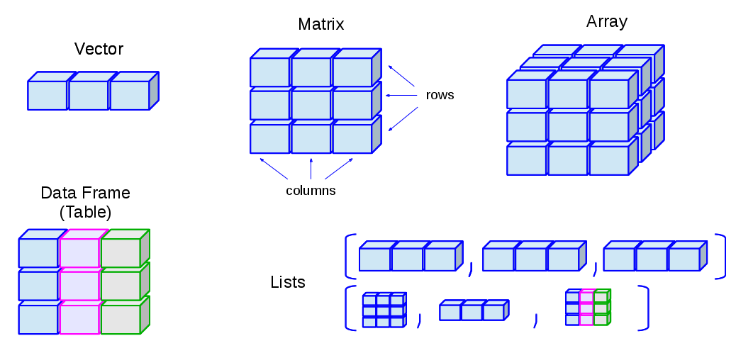
In epidemiology (and particularly field epidemiology), you will most commonly encounter data frames and vectors:

Common structure	Explanation	Example
Vectors	A container for a sequence of singular objects, all of the same class (e.g. numeric, character).	“Variables” (columns) in data frames are vectors (e.g. the column age_years).
Data Frames	Vectors (e.g. columns) that are bound together that all have the same number of rows.	linelist is a data frame.

Note that to create a vector that “stands alone” (is not part of a data frame) the function c() is used to combine the different elements. For example, if creating a vector of colors plot’s color scale: vector_of_colors <- c("blue", "red2", "orange", "grey")

Object classes

All the objects stored in R have a class which tells R how to handle the object. There are many possible classes, but common ones include:

Class	Explanation	Examples
Character	These are text/words/sentences “within quotation marks”. Math cannot be done on these objects.	“Character objects are in quotation marks”
Integer	Numbers that are whole only (no decimals)	-5, 14, or 2000
Numeric	These are numbers and can include decimals. If within quotation marks they will be considered character class.	23.1 or 14
Factor	These are vectors that have a specified order or hierarchy of values	An variable of economic status with ordered values
Date	Once R is told that certain data are Dates, these data can be manipulated and displayed in special ways. See the page on Working with dates for more information.	2018-04-12 or 15/3/1954 or Wed 4 Jan 1980
Logical	Values must be one of the two special values TRUE or FALSE (note these are not “TRUE” and “FALSE” in quotation marks)	TRUE or FALSE
data.frame	A data frame is how R stores a typical dataset. It consists of vectors (columns) of data bound together, that all have the same number of observations (rows).	The example AJS dataset named linelist_raw contains 68 variables with 300 observations (rows) each.
tibble	tibbles are a variation on data frame, the main operational difference being that they print more nicely to the console (display first 10 rows and only columns that fit on the screen)	Any data frame, list, or matrix can be converted to a tibble with as_tibble()
list	A list is like vector, but holds other objects that can be other different classes	A list could hold a single number, and a dataframe, and a vector, and even another list within it!

You can test the class of an object by providing its name to the function class(). Note: you can reference a specific column within a dataset using the $ notation to separate the name of the dataset and the name of the column.

class(linelist)         # class should be a data frame or tibble

## [1] "data.frame"

class(linelist$age)     # class should be numeric

## [1] "numeric"

class(linelist$gender)  # class should be character

## [1] "character"

Sometimes, a column will be converted to a different class automatically by R. Watch out for this! For example, if you have a vector or column of numbers, but a character value is inserted… the entire column will change to class character.

num_vector <- c(1,2,3,4,5) # define vector as all numbers
class(num_vector)          # vector is numeric class

## [1] "numeric"

num_vector[3] <- "three"   # convert the third element to a character
class(num_vector)          # vector is now character class

## [1] "character"

One common example of this is when manipulating a data frame in order to print a table - if you make a total row and try to paste/glue together percents in the same cell as numbers (e.g. 23 (40%)), the entire numeric column above will convert to character and can no longer be used for mathematical calculations.Sometimes, you will need to convert objects or columns to another class.

Function	Action
as.character()	Converts to character class
as.numeric()	Converts to numeric class
as.integer()	Converts to integer class
as.Date()	Converts to Date class - Note: see section on dates for details
factor()	Converts to factor - Note: re-defining order of value levels requires extra arguments

Likewise, there are base R functions to check whether an object IS of a specific class, such as is.numeric(), is.character(), is.double(), is.factor(), is.integer()

Here is more online material on classes and data structures in R.

Columns/Variables ($)

A column in a data frame is technically a “vector” (see table above) - a series of values that must all be the same class (either character, numeric, logical, etc).

A vector can exist independent of a data frame, for example a vector of column names that you want to include as explanatory variables in a model. To create a “stand alone” vector, use the c() function as below:

# define the stand-alone vector of character values
explanatory_vars <- c("gender", "fever", "chills", "cough", "aches", "vomit")

# print the values in this named vector
explanatory_vars

## [1] "gender" "fever"  "chills" "cough"  "aches"  "vomit"

Columns in a data frame are also vectors and can be called, referenced, extracted, or created using the $ symbol. The $ symbol connects the name of the column to the name of its data frame. In this handbook, we try to use the word “column” instead of “variable”.

# Retrieve the length of the vector age_years
length(linelist$age) # (age is a column in the linelist data frame)

By typing the name of the dataframe followed by $ you will also see a drop-down menu of all columns in the data frame. You can scroll through them using your arrow key, select one with your Enter key, and avoid spelling mistakes!

ADVANCED TIP: Some more complex objects (e.g. a list, or an epicontacts object) may have multiple levels which can be accessed through multiple dollar signs. For example epicontacts$linelist$date_onset

Access/index with brackets ([ ])

You may need to view parts of objects, also called “indexing”, which is often done using the square brackets [ ]. Using $ on a dataframe to access a column is also a type of indexing.

my_vector <- c("a", "b", "c", "d", "e", "f")  # define the vector
my_vector[5]                                  # print the 5th element

## [1] "e"

Square brackets also work to return specific parts of an returned output, such as the output of a summary() function:

# All of the summary
summary(linelist$age)

##    Min. 1st Qu.  Median    Mean 3rd Qu.    Max.    NA's 
##    0.00    6.00   13.00   16.07   23.00   84.00      86

# Just the second element of the summary, with name (using only single brackets)
summary(linelist$age)[2]

## 1st Qu. 
##       6

# Just the second element, without name (using double brackets)
summary(linelist$age)[[2]]

## [1] 6

# Extract an element by name, without showing the name
summary(linelist$age)[["Median"]]

## [1] 13

Brackets also work on data frames to view specific rows and columns. You can do this using the syntax dataframe[rows, columns]:

# View a specific row (2) from dataset, with all columns (don't forget the comma!)
linelist[2,]

# View all rows, but just one column
linelist[, "date_onset"]

# View values from row 2 and columns 5 through 10
linelist[2, 5:10] 

# View values from row 2 and columns 5 through 10 and 18
linelist[2, c(5:10, 18)] 

# View rows 2 through 20, and specific columns
linelist[2:20, c("date_onset", "outcome", "age")]

# View rows and columns based on criteria
# *** Note the dataframe must still be named in the criteria!
linelist[linelist$age > 25 , c("date_onset", "outcome", "age")]

# Use View() to see the outputs in the RStudio Viewer pane (easier to read) 
# *** Note the capital "V" in View() function
View(linelist[2:20, "date_onset"])

# Save as a new object
new_table <- linelist[2:20, c("date_onset")] 

Note that you can also achieve the above row/column indexing on data frames and tibbles using dplyr syntax (functions filter() for rows, and select() for columns). Read more about these core functions in the Cleaning data and core functions page.

To filter based on “row number”, you can use the dplyr function row_number() with open parentheses as part of a logical filtering statement. Often you will use the %in% operator and a range of numbers as part of that logical statement, as shown below. To see the first N rows, you can also use the special dplyr function head().

# View first 100 rows
linelist %>% head(100)

# Show row 5 only
linelist %>% filter(row_number() == 5)

# View rows 2 through 20, and three specific columns (note no quotes necessary on column names)
linelist %>% filter(row_number() %in% 2:20) %>% select(date_onset, outcome, age)

When indexing an object of class list, single brackets always return with class list, even if only a single object is returned. Double brackets, however, can be used to access a single element and return a different class than list.
Brackets can also be written after one another, as demonstrated below.

This visual explanation of lists indexing, with pepper shakers is humorous and helpful.

# define demo list
my_list <- list(
  # First element in the list is a character vector
  hospitals = c("Central", "Empire", "Santa Anna"),
  
  # second element in the list is a data frame of addresses
  addresses   = data.frame(
    street = c("145 Medical Way", "1048 Brown Ave", "999 El Camino"),
    city   = c("Andover", "Hamilton", "El Paso")
    )
  )

Here is how the list looks when printed to the console. See how there are two named elements:

• hospitals, a character vector
  
• addresses, a data frame of addresses

my_list

## $hospitals
## [1] "Central"    "Empire"     "Santa Anna"
## 
## $addresses
##            street     city
## 1 145 Medical Way  Andover
## 2  1048 Brown Ave Hamilton
## 3   999 El Camino  El Paso

Now we extract, using various methods:

my_list[1] # this returns the element in class "list" - the element name is still displayed

## $hospitals
## [1] "Central"    "Empire"     "Santa Anna"

my_list[[1]] # this returns only the (unnamed) character vector

## [1] "Central"    "Empire"     "Santa Anna"

my_list[["hospitals"]] # you can also index by name of the list element

## [1] "Central"    "Empire"     "Santa Anna"

my_list[[1]][3] # this returns the third element of the "hospitals" character vector

## [1] "Santa Anna"

my_list[[2]][1] # This returns the first column ("street") of the address data frame

##            street
## 1 145 Medical Way
## 2  1048 Brown Ave
## 3   999 El Camino

Remove objects

You can remove individual objects from your R environment by putting the name in the rm() function (no quote marks):

rm(object_name)

You can remove all objects (clear your workspace) by running:

rm(list = ls(all = TRUE))

3.11 Piping (%>%)

Two general approaches to working with objects are:

1. Pipes/tidyverse - pipes send an object from function to function - emphasis is on the action, not the object
   
2. Define intermediate objects - an object is re-defined again and again - emphasis is on the object

Pipes

Simply explained, the pipe operator (%>%) passes an intermediate output from one function to the next.
You can think of it as saying “then”. Many functions can be linked together with %>%.

• Piping emphasizes a sequence of actions, not the object the actions are being performed on
  
• Pipes are best when a sequence of actions must be performed on one object
  
• Pipes come from the package magrittr, which is automatically included in packages dplyr and tidyverse
• Pipes can make code more clean and easier to read, more intuitive

Read more on this approach in the tidyverse style guide

Here is a fake example for comparison, using fictional functions to “bake a cake”. First, the pipe method:

# A fake example of how to bake a cake using piping syntax

cake <- flour %>%       # to define cake, start with flour, and then...
  add(eggs) %>%   # add eggs
  add(oil) %>%    # add oil
  add(water) %>%  # add water
  mix_together(         # mix together
    utensil = spoon,
    minutes = 2) %>%    
  bake(degrees = 350,   # bake
       system = "fahrenheit",
       minutes = 35) %>%  
  let_cool()            # let it cool down

Here is another link describing the utility of pipes.

Piping is not a base function. To use piping, the magrittr package must be installed and loaded (this is typically done by loading tidyverse or dplyr package which include it). You can read more about piping in the magrittr documentation.

Note that just like other R commands, pipes can be used to just display the result, or to save/re-save an object, depending on whether the assignment operator <- is involved. See both below:

# Create or overwrite object, defining as aggregate counts by age category (not printed)
linelist_summary <- linelist %>% 
  count(age_cat)

# Print the table of counts in the console, but don't save it
linelist %>% 
  count(age_cat)

##   age_cat    n
## 1     0-4 1095
## 2     5-9 1095
## 3   10-14  941
## 4   15-19  743
## 5   20-29 1073
## 6   30-49  754
## 7   50-69   95
## 8     70+    6
## 9    <NA>   86

%<>%
This is an “assignment pipe” from the magrittr package, which pipes an object forward and also re-defines the object. It must be the first pipe operator in the chain. It is shorthand. The below two commands are equivalent:

linelist <- linelist %>%
  filter(age > 50)

linelist %<>% filter(age > 50)

Define intermediate objects

This approach to changing objects/dataframes may be better if:

• You need to manipulate multiple objects
  
• There are intermediate steps that are meaningful and deserve separate object names

Risks:

• Creating new objects for each step means creating lots of objects. If you use the wrong one you might not realize it!
  
• Naming all the objects can be confusing
  
• Errors may not be easily detectable

Either name each intermediate object, or overwrite the original, or combine all the functions together. All come with their own risks.

Below is the same fake “cake” example as above, but using this style:

# a fake example of how to bake a cake using this method (defining intermediate objects)
batter_1 <- left_join(flour, eggs)
batter_2 <- left_join(batter_1, oil)
batter_3 <- left_join(batter_2, water)

batter_4 <- mix_together(object = batter_3, utensil = spoon, minutes = 2)

cake <- bake(batter_4, degrees = 350, system = "fahrenheit", minutes = 35)

cake <- let_cool(cake)

Combine all functions together - this is difficult to read:

# an example of combining/nesting mutliple functions together - difficult to read
cake <- let_cool(bake(mix_together(batter_3, utensil = spoon, minutes = 2), degrees = 350, system = "fahrenheit", minutes = 35))

3.12 Key operators and functions

This section details operators in R, such as:

• Definitional operators
  
• Relational operators (less than, equal too..)
  
• Logical operators (and, or…)
  
• Handling missing values
  
• Mathematical operators and functions (+/-, >, sum(), median(), …)
  
• The %in% operator

Assignment operators

<-

The basic assignment operator in R is <-. Such that object_name <- value.
This assignment operator can also be written as =. We advise use of <- for general R use.
We also advise surrounding such operators with spaces, for readability.

<<-

If Writing functions, or using R in an interactive way with sourced scripts, then you may need to use this assignment operator <<- (from base R). This operator is used to define an object in a higher ‘parent’ R Environment. See this online reference.

%<>%

This is an “assignment pipe” from the magrittr package, which pipes an object forward and also re-defines the object. It must be the first pipe operator in the chain. It is shorthand, as shown below in two equivalent examples:

linelist <- linelist %>% 
  mutate(age_months = age_years * 12)

The above is equivalent to the below:

linelist %<>% mutate(age_months = age_years * 12)

%<+%

This is used to add data to phylogenetic trees with the ggtree package. See the page on Phylogenetic trees or this online resource book.

Relational and logical operators

Relational operators compare values and are often used when defining new variables and subsets of datasets. Here are the common relational operators in R:

Meaning	Operator	Example	Example Result
Equal to	==	"A" == "a"	FALSE (because R is case sensitive) Note that == (double equals) is different from = (single equals), which acts like the assignment operator <-
Not equal to	!=	2 != 0	TRUE
Greater than	>	4 > 2	TRUE
Less than	<	4 < 2	FALSE
Greater than or equal to	>=	6 >= 4	TRUE
Less than or equal to	<=	6 <= 4	FALSE
Value is missing	is.na()	is.na(7)	FALSE (see page on Missing data)
Value is not missing	!is.na()	!is.na(7)	TRUE

Logical operators, such as AND and OR, are often used to connect relational operators and create more complicated criteria. Complex statements might require parentheses ( ) for grouping and order of application.

Meaning	Operator
AND	&
OR	| (vertical bar)
Parentheses	( ) Used to group criteria together and clarify order of operations

For example, below, we have a linelist with two variables we want to use to create our case definition, hep_e_rdt, a test result and other_cases_in_hh, which will tell us if there are other cases in the household. The command below uses the function case_when() to create the new variable case_def such that:

linelist_cleaned <- linelist %>%
  mutate(case_def = case_when(
    is.na(rdt_result) & is.na(other_case_in_home)            ~ NA_character_,
    rdt_result == "Positive"                                 ~ "Confirmed",
    rdt_result != "Positive" & other_cases_in_home == "Yes"  ~ "Probable",
    TRUE                                                     ~ "Suspected"
  ))

Criteria in example above	Resulting value in new variable “case_def”
If the value for variables rdt_result and other_cases_in_home are missing	NA (missing)
If the value in rdt_result is “Positive”	“Confirmed”
If the value in rdt_result is NOT “Positive” AND the value in other_cases_in_home is “Yes”	“Probable”
If one of the above criteria are not met	“Suspected”

Note that R is case-sensitive, so “Positive” is different than “positive”…

Missing values

In R, missing values are represented by the special value NA (a “reserved” value) (capital letters N and A - not in quotation marks). If you import data that records missing data in another way (e.g. 99, “Missing”, or .), you may want to re-code those values to NA. How to do this is addressed in the [Import and export] page.

To test whether a value is NA, use the special function is.na(), which returns TRUE or FALSE.

rdt_result <- c("Positive", "Suspected", "Positive", NA)   # two positive cases, one suspected, and one unknown
is.na(rdt_result)  # Tests whether the value of rdt_result is NA

## [1] FALSE FALSE FALSE  TRUE

Read more about missing, infinite, NULL, and impossible values in the page on Missing data. Learn how to convert missing values when importing data in the page on [Import and export].

Mathematics and statistics

All the operators and functions in this page are automatically available using base R.

Mathematical operators

These are often used to perform addition, division, to create new columns, etc. Below are common mathematical operators in R. Whether you put spaces around the operators is not important.

Purpose	Example in R
addition	2 + 3
subtraction	2 - 3
multiplication	2 * 3
division	30 / 5
exponent	2^3
order of operations	( )

Mathematical functions

Purpose	Function
rounding	round(x, digits = n)
rounding	janitor::round_half_up(x, digits = n)
ceiling (round up)	ceiling(x)
floor (round down)	floor(x)
absolute value	abs(x)
square root	sqrt(x)
exponent	exponent(x)
natural logarithm	log(x)
log base 10	log10(x)
log base 2	log2(x)

Note: for round() the digits = specifies the number of decimal placed. Use signif() to round to a number of significant figures.

Scientific notation

The likelihood of scientific notation being used depends on the value of the scipen option.

From the documentation of ?options: scipen is a penalty to be applied when deciding to print numeric values in fixed or exponential notation. Positive values bias towards fixed and negative towards scientific notation: fixed notation will be preferred unless it is more than ‘scipen’ digits wider.

If it is set to a low number (e.g. 0) it will be “turned on” always. To “turn off” scientific notation in your R session, set it to a very high number, for example:

# turn off scientific notation
options(scipen=999)

Rounding

DANGER: round() uses “banker’s rounding” which rounds up from a .5 only if the upper number is even. Use round_half_up() from janitor to consistently round halves up to the nearest whole number. See this explanation

# use the appropriate rounding function for your work
round(c(2.5, 3.5))

## [1] 2 4

janitor::round_half_up(c(2.5, 3.5))

## [1] 3 4

Statistical functions

CAUTION: The functions below will by default include missing values in calculations. Missing values will result in an output of NA, unless the argument na.rm = TRUE is specified. This can be written shorthand as na.rm = T.

Objective	Function
mean (average)	mean(x, na.rm=T)
median	median(x, na.rm=T)
standard deviation	sd(x, na.rm=T)
quantiles*	quantile(x, probs)
sum	sum(x, na.rm=T)
minimum value	min(x, na.rm=T)
maximum value	max(x, na.rm=T)
range of numeric values	range(x, na.rm=T)
summary**	summary(x)

Notes:

• *quantile(): x is the numeric vector to examine, and probs = is a numeric vector with probabilities within 0 and 1.0, e.g c(0.5, 0.8, 0.85)
• **summary(): gives a summary on a numeric vector including mean, median, and common percentiles

DANGER: If providing a vector of numbers to one of the above functions, be sure to wrap the numbers within c() .

# If supplying raw numbers to a function, wrap them in c()
mean(1, 6, 12, 10, 5, 0)    # !!! INCORRECT !!!  

## [1] 1

mean(c(1, 6, 12, 10, 5, 0)) # CORRECT

## [1] 5.666667

Other useful functions

Objective	Function	Example
create a sequence	seq(from, to, by)	seq(1, 10, 2)
repeat x, n times	rep(x, ntimes)	rep(1:3, 2) or rep(c("a", "b", "c"), 3)
subdivide a numeric vector	cut(x, n)	cut(linelist$age, 5)
take a random sample	sample(x, size)	sample(linelist$id, size = 5, replace = TRUE)

%in%

A very useful operator for matching values, and for quickly assessing if a value is within a vector or dataframe.

my_vector <- c("a", "b", "c", "d")

"a" %in% my_vector

## [1] TRUE

"h" %in% my_vector

## [1] FALSE

To ask if a value is not %in% a vector, put an exclamation mark (!) in front of the logic statement:

# to negate, put an exclamation in front
!"a" %in% my_vector

## [1] FALSE

!"h" %in% my_vector

## [1] TRUE

%in% is very useful when using the dplyr function case_when(). You can define a vector previously, and then reference it later. For example:

affirmative <- c("1", "Yes", "YES", "yes", "y", "Y", "oui", "Oui", "Si")

linelist <- linelist %>% 
  mutate(child_hospitaled = case_when(
    hospitalized %in% affirmative & age < 18 ~ "Hospitalized Child",
    TRUE                                      ~ "Not"))

Note: If you want to detect a partial string, perhaps using str_detect() from stringr, it will not accept a character vector like c("1", "Yes", "yes", "y"). Instead, it must be given a regular expression - one condensed string with OR bars, such as “1|Yes|yes|y”. For example, str_detect(hospitalized, "1|Yes|yes|y"). See the page on Characters and strings for more information.

You can convert a character vector to a named regular expression with this command:

affirmative <- c("1", "Yes", "YES", "yes", "y", "Y", "oui", "Oui", "Si")
affirmative

## [1] "1"   "Yes" "YES" "yes" "y"   "Y"   "oui" "Oui" "Si"

# condense to 
affirmative_str_search <- paste0(affirmative, collapse = "|")  # option with base R
affirmative_str_search <- str_c(affirmative, collapse = "|")   # option with stringr package

affirmative_str_search

## [1] "1|Yes|YES|yes|y|Y|oui|Oui|Si"

3.13 Errors & warnings

This section explains:

• The difference between errors and warnings
  
• General syntax tips for writing R code
  
• Code assists

Common errors and warnings and troubleshooting tips can be found in the page on [Errors and help].

Error versus Warning

When a command is run, the R Console may show you warning or error messages in red text.

• A warning means that R has completed your command, but had to take additional steps or produced unusual output that you should be aware of.

• An error means that R was not able to complete your command.

Look for clues:

• The error/warning message will often include a line number for the problem.

• If an object “is unknown” or “not found”, perhaps you spelled it incorrectly, forgot to call a package with library(), or forgot to re-run your script after making changes.

If all else fails, copy the error message into Google along with some key terms - chances are that someone else has worked through this already!

General syntax tips

A few things to remember when writing commands in R, to avoid errors and warnings:

• Always close parentheses - tip: count the number of opening “(” and closing parentheses “)” for each code chunk
• Avoid spaces in column and object names. Use underscore ( _ ) or periods ( . ) instead
• Keep track of and remember to separate a function’s arguments with commas
• R is case-sensitive, meaning Variable_A is different from variable_A

Code assists

Any script (RMarkdown or otherwise) will give clues when you have made a mistake. For example, if you forgot to write a comma where it is needed, or to close a parentheses, RStudio will raise a flag on that line, on the right side of the script, to warn you.